Hanze

Go back to the main page
Go back to the Excel overview page

Files used on this page:

file01_KEGG_DRUG_ATC_PROPERTIES_PED_FP.csv

Excel: Data Cleaning

Introduction

In data science, data is typically organized in a structured format, such as a table or a spreadsheet. This allows for easy manipulation and analysis of the data.

However, a lot of data coming from external sources such as lab equipment and factory equipment will not be directly suitable for data analysis. In that case, data cleaning en reorganization might me required.

Excel lags behind Python and R in capabilities of data reorganization and cleaning. Nevertheless, Excel has some features that are worth explaining. We will discuss them here.

Text to column feature

If your csv data import fails, you can manually parse your text to various columns. Take a look at the following example (source):

Or here as csv file.

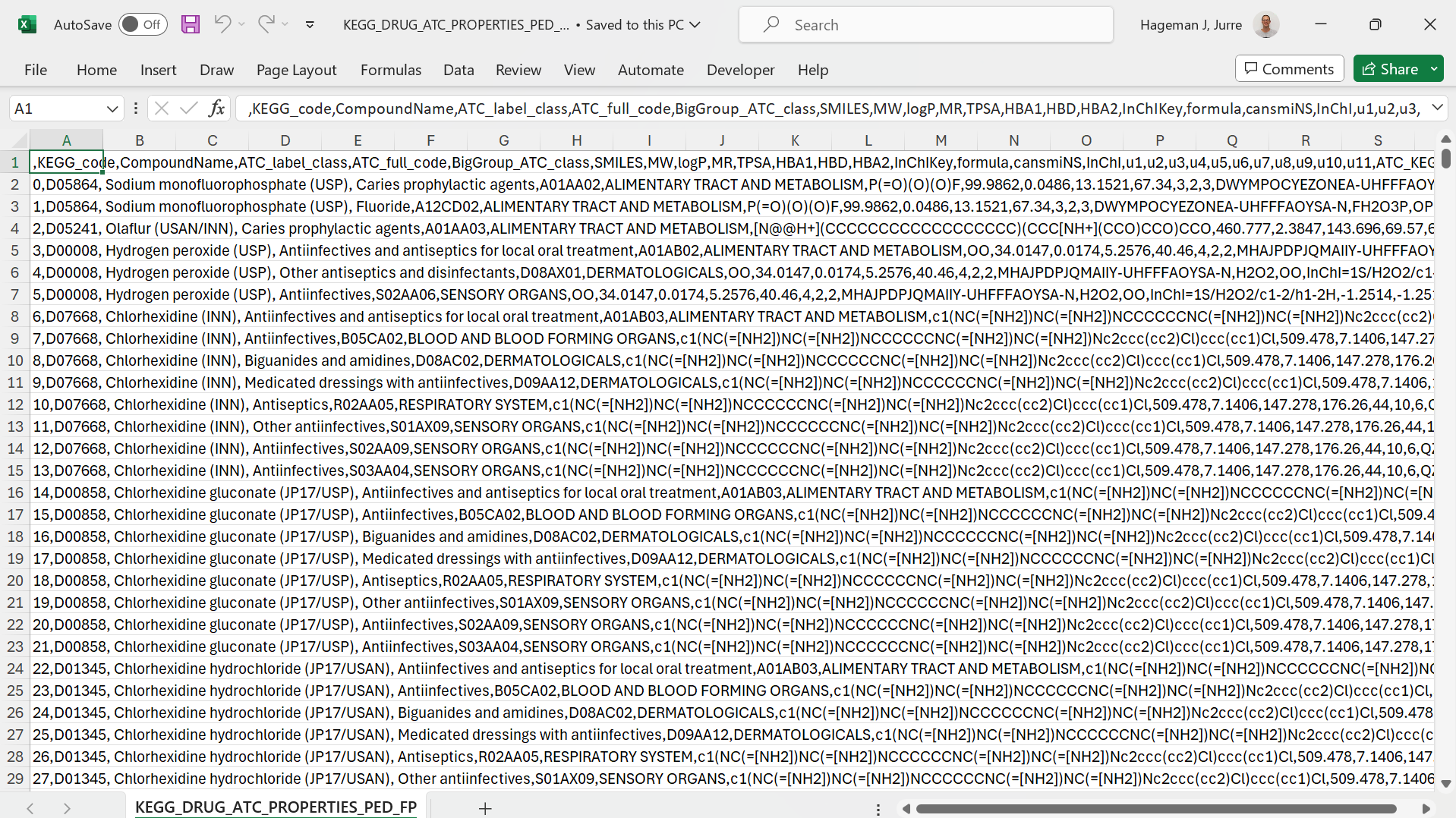food _{Figure 1: All data in a single column}

As you can see, all data is loaded in the first column. You can use the text to columns functionality that can be found on the data tab in the ribbon.

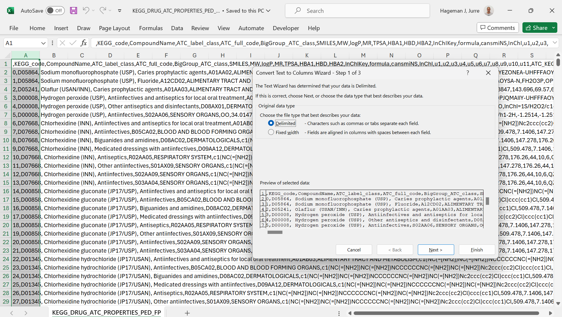food2 _{Figure 2: Select the delimiter}

Here the correct column separator is selected to parse the text. The result is as follows:

food3 _{Figure 3: Text separated to columns}

As you can see from the picture above, the text is now separated in different columns based on the correct column separator.

Remove duplicates

On the data tab in the ribbon, you will find an option to remove duplicate rows:

_{Figure 4: Remove duplicates feature}

As can be seen from the picture below, row ID 2 is a duplicate.

duplicates _{Figure 5: Two duplicate rows}

You can select columns to compare. In the case below, all columns were selected.

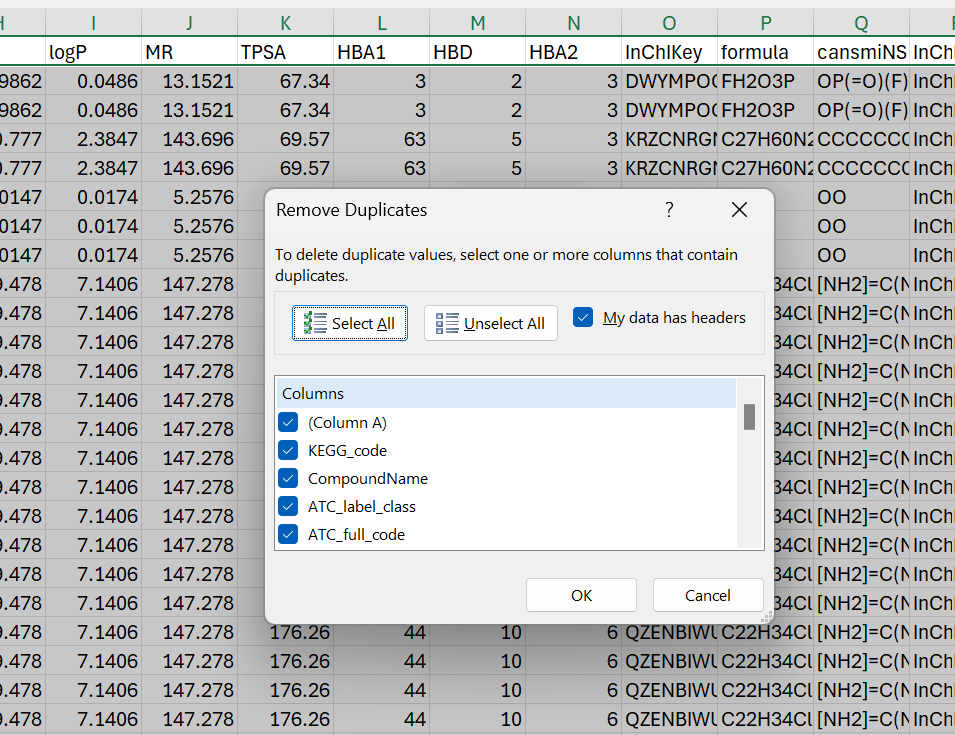duplicates _{Figure 6: Columns selected to compare}

Excel reports the removal of 1 duplicate row.

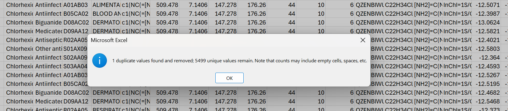duplicates _{Figure 7: 1 duplicate value removed.}

And the result is 1 duplicate row removed.

duplicates _{Figure 8: 1 duplicate row removed.}

Trimming text

Often, data will contain extra whitespace such as spaces. Extra spaces are notoriously difficult to spot, especially those at the end. Those extra spaces may interfere with later analysis.

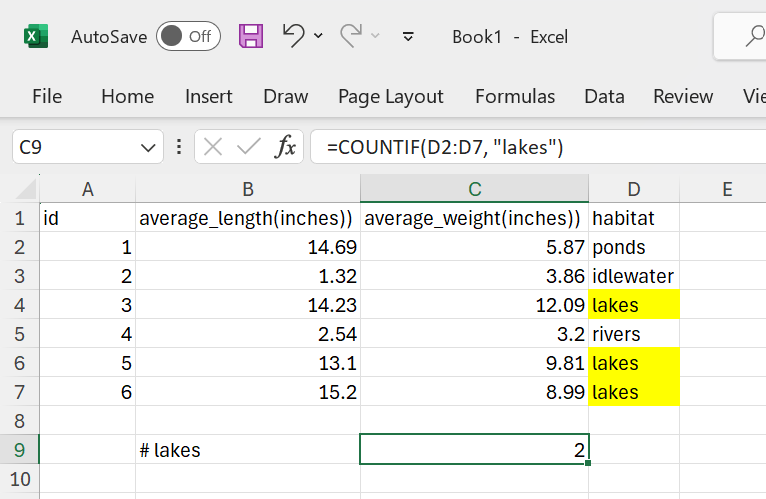extra spaces _{Figure 9: Only 2 “lakes” counted as one cell contains “lakes “ with a tailing space.}

The TRIM function will remove trailing whitespace:

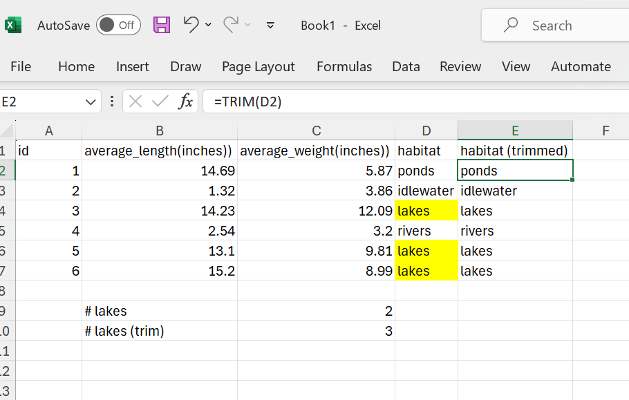extra spaces _{Figure 10: The TRIM function in action.}

As a result, the tailing whitespace is now removed and the COUNTIF function returns the expected result.

Find and replace

Find and replace is useful to clean data. This example shows some HTML tags in cells:

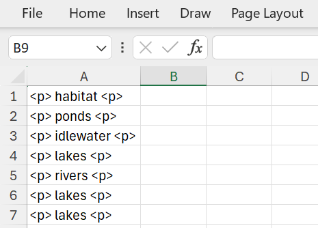find replace _{Figure 11: HTML tags in cells.}

Removing them is easy using find and replace:

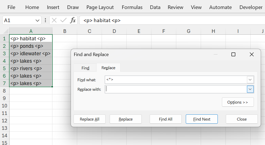find replace _{Figure 12: Remove HTML tags in cells.}

The * is a wildcard that represents any text. Note that you do not need to explicitly specify an empty string in the replace with field. Excel will take care of this.

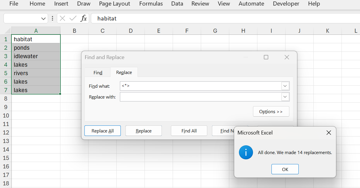find replace _{Figure 13: HTML tags removed.}

There are some other handy functions that work on strings that can help you:

Function	Explanation
FIND	FIND and FINDB locate one text string within a second text string, and return the number of the starting position of the first text string from the first character of the second text string. FIND is case sensitive.
SEARCH	The SEARCH and SEARCHB functions locate one text string within a second text string, and return the number of the starting position of the first text string from the first character of the second text string. SEARCH is not case sensitive.
REPLACE	REPLACE replaces part of a text string, based on the number of characters you specify, with a different text string.
SUBSTITUTE	Substitutes new_text for old_text in a text string. Use SUBSTITUTE when you want to replace specific text in a text string; use REPLACE when you want to replace any text that occurs in a specific location in a text string.
LEFT	LEFT returns the first character or characters in a text string, based on the number of characters you specify.
RIGHT	RIGHT returns the last character or characters in a text string, based on the number of characters you specify.
LEN	LEN returns the number of characters in a text string.
MID	MID returns a specific number of characters from a text string, starting at the position you specify, based on the number of characters you specify.

Splitting and concatenating strings

Sometimes tou want to split data on a certain character:

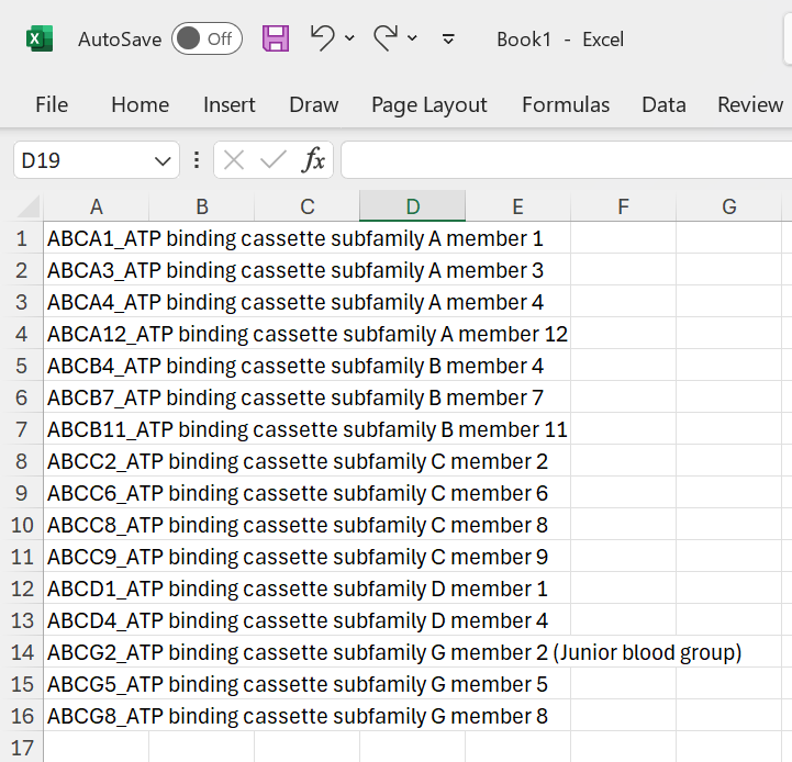split _{Figure 14: Split on a character.}

The TEXTSPLIT function can handle this:

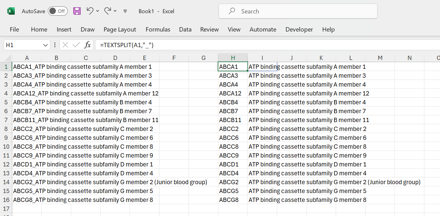split _{Figure 15: Split on a character.}

The reciprocal function is CONCAT. Here you can see it in action:

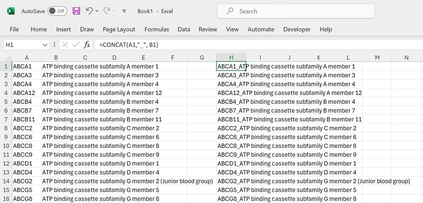concat _{Figure 16: Concatenate text strings.}

Dealing with missing data

Finding missing data

Often, data analysts are dealing with missing data in datasets. Data fields may be simply empty, contain a dash (-) or may contain an #N/A error. There are various approaches one can take when dealing with missing data. For example, you can throw out all the data for any sample missing one or more data elements. However, be aware that missing data might not be randomly distributed.

The approaches that can be taken are:

Delete the samples (rows) with one or more missing data elements;
Input values for missing data elements;
Remove a complete variable (column) that has a lot of missing values.

Plain Excel does not have a lot of support to drop rows or columns with missing values. A simple approach would be to create a table, filter the data and then manually delete rows that contain empty values.

You can find empty cells using the COUNTBLANK function:

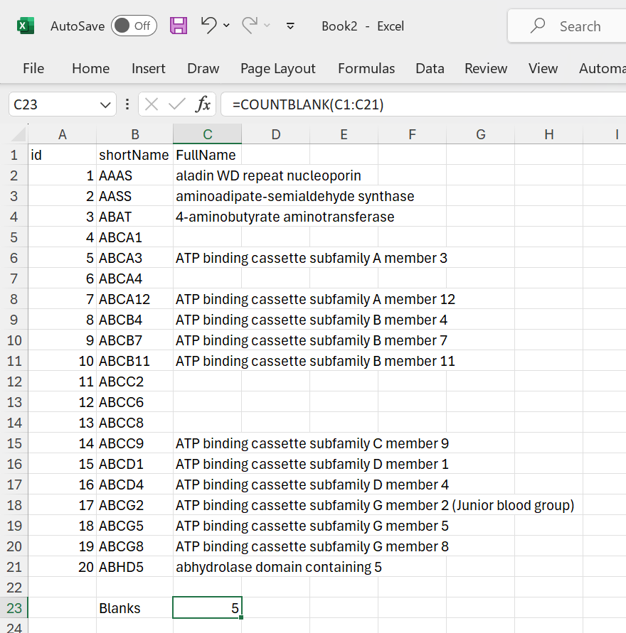countblank _{Figure 17: Counting blank cells.}

Likewise, it is also possible to count the #N/A values:

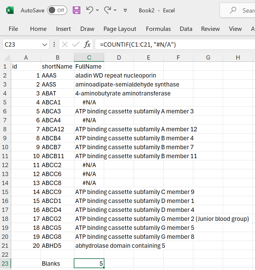count na _{Figure 18: Counting #N/A cells.}

Or check if they are equal to #N/A using the ISNA function:

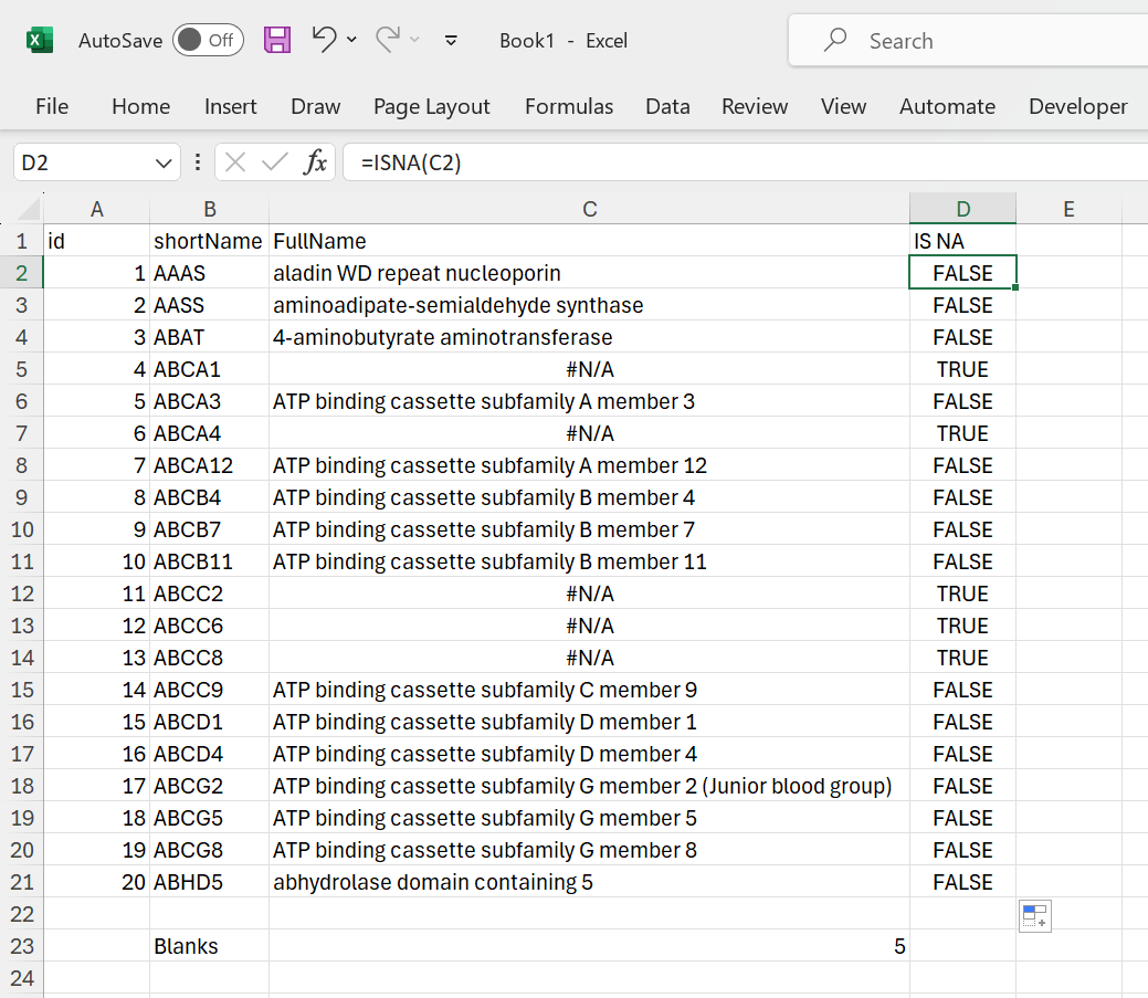count na _{Figure 19: Validate if cell equals #N/A.}

In addition to counting missing data as #N/A in the FullName column, we can also identify the item in the shortName column using XLOOKUP:

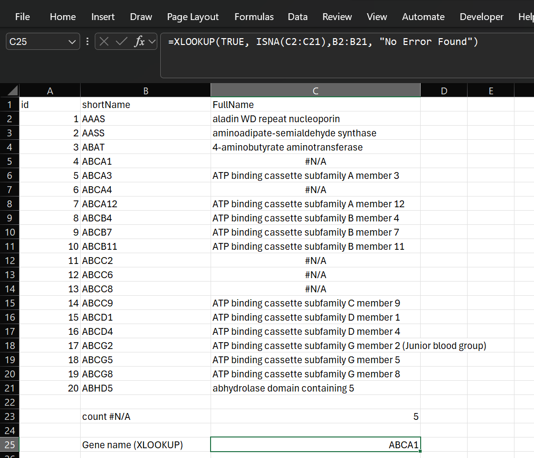xlookup _{Figure 20: Identify the gene with an #N/A error using XLOOKUP.}

As we can not directly search for an #N/A we needed to use the expression:

=XLOOKUP(TRUE, ISNA(lookup_array), return_array)

In addition, XLOOKUP can only find the first instance of an #N/A value. Therefore, it is better to use the FILTER function to filter for rows with an #N/A:

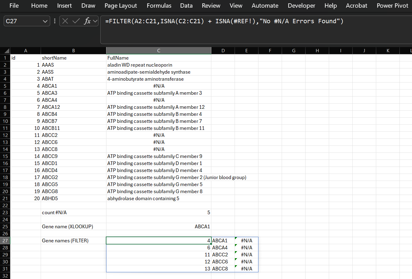xlookup _{Figure 21: Identify rows with an #N/A error using FILTER.}

Note that the FILTER function is an array function and returns it’s results across multiple cells.

Bulk delete rows with missing values

There are multiple ways to do this. Two are explained here:

Using Go To Special on a Specific Column

This method is quick, but it’s important to select only the column you want to check for blanks to prevent Excel from trying to select blank cells in your other data columns.

Select the Key Column: Click the column letter (e.g., click C if you want to check Column C) to select the entire column that must not contain blank values.
Open Go To Special: Press Ctrl + G (or F5), then click the Special… button.
Select Blanks: Choose the Blanks radio button and click OK.
Excel selects all empty cells only in the column you selected (e.g., all blank cells in Column C).
Delete Entire Rows: Press Ctrl + - (minus sign) to open the Delete dialog box.
Choose Entire Row: Select Entire row and click OK.

Result: Any row containing a selected blank cell in your key column will be deleted, regardless of whether other cells in that row contained data.

Using Filter on a Specific Column

This is often the safest and most visual method, as you can review the rows to be deleted before you execute the action.

Apply Filter: Select your entire dataset (including the header row), go to the Data tab, and click Filter (or use the shortcut Ctrl + Shift + L).
Filter for Blanks in Key Column: Click the filter arrow in the header of the specific column you want to check for missing values.
Deselect All and Select Blanks:
Uncheck the (Select All) box.
Scroll to the very bottom and check the (Blanks) option.
Click OK.
Only rows with a blank value in that specific column will now be visible.
Select and Delete Visible Rows:
Select all the visible rows of data (excluding the header row).
Right-click on any selected row number and choose Delete Row.
Clear Filter: Go back to the Data tab and click the Clear button to display all your remaining data.

Delete Blank Rows Using Power Query

The primary advantage of Power Query is that it is dynamic: if you add new data to your source table, you simply click “Refresh” on the output table, and the blank rows are instantly removed.

Step 1: Load Data into Power Query Editor

Select any cell in your data table.
Go to the Data tab on the Excel ribbon.
In the Get & Transform Data group, click From Table/Range.
If prompted, confirm the range and ensure “My table has headers” is checked, then click OK.
This opens the Power Query Editor window.

Step 2: Filter the Specific Column for Blanks

In the Power Query Editor, navigate to the header of the specific column (e.g., “Customer ID”) that you want to check for blank values.

Click the down arrow on that column header.
In the text filter menu, uncheck the box for (null) (or (Blanks)).

Working with #N/A

In any case, it is best to convert cells with “empty” values (whether it is truly blank, contains a dash or any other character to mark empty) to #N/A. #N/A is the error value of Excel that means “no value is available.” To avoid accidentally including empty cells in your calculations, enter #N/A in the cells where you are missing information. (A formula that references a cell that contains #N/A will return the #N/A error value). Read more about #N/A here.

Use simply find and replace to insert #N/A in “empty” cells.

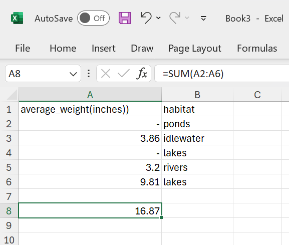dealing with na _{Figure 22: The SUM function still works, ignoring missing data.}

As you can see, the SUM function still works. This might look appealing at first sight, but it also can cause a lot of troubles when you deal with larger datasets. It masks missing data!

So convert to #N/A:

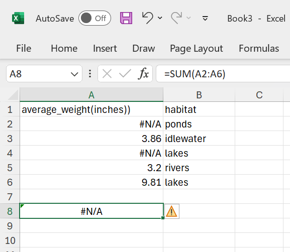dealing with na _{Figure 23: The SUM function does not work when #N/A is included.}

As a result, the SUM function does not work. It does notify you that there are missing data. Now you can deal with the #N/A using the SUMIF function:

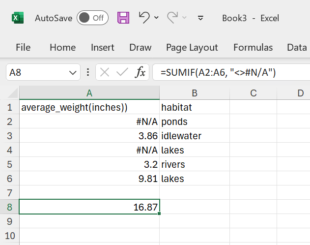dealing with na _{Figure 24: The SUMIF function does work when #N/A is included.}

In the above example, <> is a shorthand for the NOT operator. So the formula reads as: Only sum cells that are not equal to #N/A and ignore the #N/A's. This is a strategy that is very similar to what is used in R and Python. Your are dealing with missing data in an explicit way instead of implicit.

Like many things in real life, datasets are often imperfect. Very often, data points will be missing. This is just reality and there is not much that you can do about the fact that you will encounter missing data. What is important though, is how you deal with missing data. Make it explicit that data is missing in your analysis and deal with it in a transparent way.

Go back to the main page
Go back to the Excel overview page
⬆️ Back to Top

This web page is distributed under the terms of the Creative Commons Attribution License which permits unrestricted use, distribution, and reproduction in any medium, provided the original author and source are credited. Creative Commons License: CC BY-SA 4.0.

data_analysis_bml

BML data analysis